结构方程模型R语言实战教程

2024年02月28日

文章目录

1. 安装
2. 数据
3. 测量模型的设定
4. 结构模型的设定
5. 估计结果
6. Bootstrapping方法用于估计参数的显著性
7. 汇报结果
8. 描述性统计
9. 参考文献

SEMinR 为创建和估计结构方程模型 (SEM) 非常容易的使用方法。 SEMinR 集成了 SmartPLS 具有的偏最小二乘路径建模 (PLS-PM) 进行估计，也可以使用 LISREL 和 AMOS 的基于协方差的结构方程模型 (CBSEM) 进行估计，还支持反应性测量模型的验证性因素分析 (CFA)。SEMinR 中 CBSEM 和 CFA 估计都使用 Lavaan 软件包。

SEMinR 有如下特点：

使用一种通俗易懂语言，用于在 R 中构建和估计结构方程模型
可以使用基于方差的 PLS 估计和基于协方差的 SEM 估计来对潜变量结构进行建模
高级函数可快速指定交互作用、高阶结构和结构路径

SEMinR 使用自己的 PLS-PM 估计引擎，并与 Lavaan 软件包集成以进行 CBSEM/CFA 估计。它还带来了其他软件包或软件中没有的一些方法。

安装

使用如下代码安装 SEMinR ，它是R的包，所以你需要在R中运行如下代码：

1	install.packages("seminr")

注意seminr是使用R4.3.3编译的, 你的R版本不能低于这个版本.

然后加载包：

1	library(seminr)

数据

你需要从任何数据文件中加载数据到数据框（data.frame）。列名必须是测量项目的名称。重要提示：避免在列名称中使用星号“*”（这些是为交互术语保留的）。

我们的教程使用的是 seminr 自带的数据集 mobi, 可以使用data方法加载数据, 如下:

1 2	df=data('mobi') head(mobi)

输出(html):

A data.frame: 6 × 24
	CUEX1	CUEX2	CUEX3	CUSA1	CUSA2	CUSA3	CUSCO	CUSL1	CUSL2	CUSL3	⋯	IMAG5	PERQ1	PERQ2	PERQ3	PERQ4	PERQ5	PERQ6	PERQ7	PERV1	PERV2
	<int>	<int>	<int>	<int>	<int>	<int>	<int>	<int>	<int>	<int>	⋯	<int>	<int>	<int>	<int>	<int>	<int>	<int>	<int>	<int>	<int>
1	7	7	6	6	4	7	7	6	5	6	⋯	4	7	6	4	7	6	5	5	2	3
2	10	10	9	10	10	8	10	10	2	10	⋯	9	10	9	10	10	9	10	10	10	10
3	7	7	7	8	7	7	6	6	2	7	⋯	7	7	8	5	7	8	7	7	7	7
4	7	10	5	10	10	10	5	10	4	10	⋯	10	8	10	10	8	4	5	8	5	5
5	8	7	10	10	8	8	5	10	3	8	⋯	9	10	9	8	10	9	9	8	6	6
6	10	9	7	8	7	7	8	10	3	10	⋯	9	9	10	9	10	8	9	9	10	10

mobi 数据框（也可在 semPLS R 软件包中找到）该数据集来自适用于移动电话市场的欧洲客户满意度指数 (ECSI) 测量工具（Tenenhaus 等人，2005 年）。

下面是一些描述性统计:

1	dim(mobi) # 有250个样本, 24个变量

输出(html):

1	summary(mobi)

输出(plain):
CUEX1 CUEX2 CUEX3 CUSA1
Min. : 1.00 Min. : 1.000 Min. : 1.000 Min. : 4.000
1st Qu.: 7.00 1st Qu.: 7.000 1st Qu.: 6.000 1st Qu.: 7.000
Median : 8.00 Median : 8.000 Median : 8.000 Median : 8.000
Mean : 7.58 Mean : 7.532 Mean : 7.424 Mean : 7.988
3rd Qu.: 8.00 3rd Qu.: 9.000 3rd Qu.: 9.000 3rd Qu.: 9.000
Max. :10.00 Max. :10.000 Max. :10.000 Max. :10.000
CUSA2 CUSA3 CUSCO CUSL1
Min. : 1.000 Min. : 1.000 Min. : 1.000 Min. : 1.000
1st Qu.: 6.000 1st Qu.: 7.000 1st Qu.: 6.000 1st Qu.: 6.000
Median : 7.000 Median : 7.000 Median : 7.000 Median : 8.000
Mean : 7.128 Mean : 7.316 Mean : 7.068 Mean : 7.452
3rd Qu.: 8.000 3rd Qu.: 8.000 3rd Qu.: 9.000 3rd Qu.:10.000
Max. :10.000 Max. :10.000 Max. :10.000 Max. :10.000
CUSL2 CUSL3 IMAG1 IMAG2
Min. : 1.000 Min. : 1.000 Min. : 1.00 Min. : 1.00
1st Qu.: 3.000 1st Qu.: 7.000 1st Qu.: 7.00 1st Qu.: 7.00
Median : 4.000 Median : 8.000 Median : 8.00 Median : 8.00
Mean : 4.988 Mean : 7.668 Mean : 7.64 Mean : 7.78
3rd Qu.: 6.750 3rd Qu.:10.000 3rd Qu.: 9.00 3rd Qu.: 9.00
Max. :10.000 Max. :10.000 Max. :10.00 Max. :10.00
IMAG3 IMAG4 IMAG5 PERQ1
Min. : 1.000 Min. : 1.000 Min. : 1.000 Min. : 2.000
1st Qu.: 5.000 1st Qu.: 7.000 1st Qu.: 7.000 1st Qu.: 7.000
Median : 7.000 Median : 8.000 Median : 8.000 Median : 8.000
Mean : 6.744 Mean : 7.588 Mean : 7.932 Mean : 7.944
3rd Qu.: 8.000 3rd Qu.: 9.000 3rd Qu.: 9.000 3rd Qu.: 9.000
Max. :10.000 Max. :10.000 Max. :10.000 Max. :10.000
PERQ2 PERQ3 PERQ4 PERQ5
Min. : 1.000 Min. : 1.0 Min. : 1.000 Min. : 3.000
1st Qu.: 6.000 1st Qu.: 7.0 1st Qu.: 7.000 1st Qu.: 7.000
Median : 7.000 Median : 8.0 Median : 8.000 Median : 8.000
Mean : 7.192 Mean : 7.7 Mean : 7.916 Mean : 7.872
3rd Qu.: 8.000 3rd Qu.: 9.0 3rd Qu.: 9.000 3rd Qu.: 9.000
Max. :10.000 Max. :10.0 Max. :10.000 Max. :10.000
PERQ6 PERQ7 PERV1 PERV2
Min. : 1.000 Min. : 1.000 Min. : 1.000 Min. : 1.000
1st Qu.: 7.000 1st Qu.: 7.000 1st Qu.: 5.000 1st Qu.: 6.000
Median : 8.000 Median : 8.000 Median : 6.000 Median : 7.000
Mean : 7.776 Mean : 7.592 Mean : 6.156 Mean : 6.916
3rd Qu.: 9.000 3rd Qu.: 9.000 3rd Qu.: 8.000 3rd Qu.: 8.000
Max. :10.000 Max. :10.000 Max. :10.000 Max. :10.000

测量模型的设定

“multi_items”这个函数非常有用, 我么可以使用”multi_items”来生成连续变化的变量名, 例如:

1	multi_items("IMAG", 1:5)

输出(html):

'IMAG1'
'IMAG2'
'IMAG3'
'IMAG4'
'IMAG5'

1
2
3

# 不连续的变量名

multi_items("IMAG", c(1, 3:5))

输出(html):

'IMAG1'
'IMAG3'
'IMAG4'
'IMAG5'

“composite”这个函数顾名思义, 就是生成一个”构建”, 即形成性潜变量, 形成性只能在pls-sem中使用, 也就是说像AMOS这样的软件是不支持的, 例如:

1 2	# 构建一个潜变量, 名为IMAG, 有五个题目, 分别是: 'IMAG1''IMAG2''IMAG3''IMAG4''IMAG5' composite("IMAG", multi_items("IMAG", 1:5))

输出(html):

'IMAG'
'IMAG1'
'A'
'IMAG'
'IMAG2'
'A'
'IMAG'
'IMAG3'
'A'
'IMAG'
'IMAG4'
'A'
'IMAG'
'IMAG5'
'A'

如果你的潜变量是反应性的, 即由反应性指标构成, 那么我们需要使用 “reflective” 方法, 基于协方差矩阵的结构方程模型只能支持反应性的指标:

1	reflective("IMAG", multi_items("IMAG", 1:5))

输出(html):

'IMAG'
'IMAG1'
'C'
'IMAG'
'IMAG2'
'C'
'IMAG'
'IMAG3'
'C'
'IMAG'
'IMAG4'
'C'
'IMAG'
'IMAG5'
'C'

定义测量模型使用”constructs”, 例如:

measurements <- constructs(
  composite("Image",        multi_items("IMAG", 1:5)),
  composite("Expectation",  multi_items("CUEX", 1:3)),
  composite("Value",        multi_items("PERV", 1:2)),
  composite("Satisfaction", multi_items("CUSA", 1:3)),
  interaction_term(iv = "Image", moderator = "Expectation")
)

measurement

输出(html):

$composite

'Image'
'IMAG1'
'A'
'Image'
'IMAG2'
'A'
'Image'
'IMAG3'
'A'
'Image'
'IMAG4'
'A'
'Image'
'IMAG5'
'A'

$composite

'Expectation'
'CUEX1'
'A'
'Expectation'
'CUEX2'
'A'
'Expectation'
'CUEX3'
'A'

$composite

'Value'
'PERV1'
'A'
'Value'
'PERV2'
'A'

$composite

'Satisfaction'
'CUSA1'
'A'
'Satisfaction'
'CUSA2'
'A'
'Satisfaction'
'CUSA3'
'A'

$scaled_interaction

structure(function (data, measurement_model, structural_model, 
    ints, ...) 
{
    interaction_name <- paste(iv, moderator, sep = "*")
    iv1_items <- measurement_model[measurement_model[, "construct"] == 
        iv, "measurement"]
    iv2_items <- measurement_model[measurement_model[, "construct"] == 
        moderator, "measurement"]
    iv1_data <- as.data.frame(scale(data[iv1_items]))
    iv2_data <- as.data.frame(scale(data[iv2_items]))
    multiples_list <- lapply(iv1_data, mult, iv2_data)
    interaction_data <- do.call("cbind", multiples_list)
    colnames(interaction_data) <- as.vector(sapply(iv1_items, 
        name_items, iv2_items))
    intxn_mm <- matrix(measure_interaction(interaction_name, 
        interaction_data, weights), ncol = 3, byrow = TRUE)
    return(list(name = interaction_name, data = interaction_data, 
        mm = intxn_mm))
}, class = c("function", "interaction", "scaled_interaction"))

我们使用了interaction_term来定义交互项, 它是用来检验调节效应的, 下面我们定义结构模型:

结构模型的设定

“paths”就是路径的意思, 我们用这个方法可以定义一条或者多条路径, 它的from参数就是路径的起点, 它的to参数就是路径的终点, “relationships”函数用于将所有的路径组合起来构成结构模型:


structure <- relationships(
  paths(from = c("Image", "Expectation", "Image*Expectation"), to = "Value"),
  paths(from = "Value", to = "Satisfaction")
)

估计结果

结构方程由测量模型和结构模型构成, 有了上面的模型, 我们可以计算结果了.

假如我们想使用最小二乘法估计结构方程, 那么我们这样做:

pls_model <- estimate_pls(data = mobi, 
                          measurement_model = measurements, 
                          structural_model = structure)
summary(pls_model)

输出(stream):
Generating the seminr model All 250 observations are valid.

输出(plain):

Results from package seminr (2.3.2)

Path Coefficients:
Value Satisfaction
R^2 0.321 0.376
AdjR^2 0.313 0.373
Image 0.459 .
Expectation 0.143 .
Image*Expectation -0.143 .
Value . 0.613

Reliability:
alpha rhoC AVE rhoA
Image 0.723 0.817 0.476 0.753
Expectation 0.452 0.727 0.474 0.466
Image*Expectation 0.802 0.256 0.141 1.000
Value 0.824 0.918 0.848 0.859
Satisfaction 0.779 0.870 0.692 0.806

Alpha, rhoC, and rhoA should exceed 0.7 while AVE should exceed 0.5

1
2
3

# 使用bootstrap的方法来计算路径系数的显著性和置信区间
boot_estimates <- bootstrap_model(pls_model, nboot = 1000, cores = 2)
summary(boot_estimates)

输出(stream):
Bootstrapping model using seminr... SEMinR Model successfully bootstrapped

输出(plain):

Results from Bootstrap resamples: 1000

Bootstrapped Structural Paths:
Original Est. Bootstrap Mean Bootstrap SD T Stat.
Image -> Value 0.459 0.436 0.069 6.611
Expectation -> Value 0.143 0.149 0.074 1.924
Image*Expectation -> Value -0.143 -0.015 0.178 -0.803
Value -> Satisfaction 0.613 0.615 0.059 10.462
2.5% CI 97.5% CI
Image -> Value 0.301 0.572
Expectation -> Value -0.001 0.289
Image*Expectation -> Value -0.250 0.251
Value -> Satisfaction 0.485 0.714

Bootstrapped Weights:
Original Est. Bootstrap Mean Bootstrap SD
IMAG1 -> Image 0.322 0.316 0.042
IMAG2 -> Image 0.223 0.223 0.055
IMAG3 -> Image 0.275 0.273 0.046
IMAG4 -> Image 0.387 0.388 0.050
IMAG5 -> Image 0.220 0.217 0.055
CUEX1 -> Expectation 0.562 0.551 0.088
CUEX2 -> Expectation 0.344 0.335 0.135
CUEX3 -> Expectation 0.524 0.517 0.114
PERV1 -> Value 0.476 0.477 0.020
PERV2 -> Value 0.607 0.606 0.027
CUSA1 -> Satisfaction 0.327 0.328 0.032
CUSA2 -> Satisfaction 0.391 0.390 0.024
CUSA3 -> Satisfaction 0.477 0.477 0.033
IMAG1*CUEX1 -> Image*Expectation -0.262 0.077 0.180
IMAG1*CUEX2 -> Image*Expectation -0.211 0.083 0.175
IMAG1*CUEX3 -> Image*Expectation 0.088 0.085 0.157
IMAG2*CUEX1 -> Image*Expectation 0.322 0.081 0.216
IMAG2*CUEX2 -> Image*Expectation 0.199 0.043 0.182
IMAG2*CUEX3 -> Image*Expectation 0.374 0.075 0.235
IMAG3*CUEX1 -> Image*Expectation -0.030 0.081 0.160
IMAG3*CUEX2 -> Image*Expectation -0.065 0.061 0.144
IMAG3*CUEX3 -> Image*Expectation 0.396 0.087 0.218
IMAG4*CUEX1 -> Image*Expectation -0.128 0.084 0.143
IMAG4*CUEX2 -> Image*Expectation -0.038 0.079 0.139
IMAG4*CUEX3 -> Image*Expectation 0.203 0.085 0.162
IMAG5*CUEX1 -> Image*Expectation -0.264 0.010 0.207
IMAG5*CUEX2 -> Image*Expectation 0.071 0.032 0.162
IMAG5*CUEX3 -> Image*Expectation 0.200 0.047 0.193
T Stat. 2.5% CI 97.5% CI
IMAG1 -> Image 7.620 0.235 0.401
IMAG2 -> Image 4.057 0.115 0.330
IMAG3 -> Image 5.916 0.182 0.365
IMAG4 -> Image 7.801 0.300 0.495
IMAG5 -> Image 4.030 0.096 0.314
CUEX1 -> Expectation 6.378 0.369 0.721
CUEX2 -> Expectation 2.545 0.017 0.569
CUEX3 -> Expectation 4.617 0.299 0.748
PERV1 -> Value 24.180 0.435 0.512
PERV2 -> Value 22.544 0.560 0.663
CUSA1 -> Satisfaction 10.275 0.260 0.382
CUSA2 -> Satisfaction 16.288 0.341 0.433
CUSA3 -> Satisfaction 14.513 0.422 0.553
IMAG1*CUEX1 -> Image*Expectation -1.457 -0.278 0.388
IMAG1*CUEX2 -> Image*Expectation -1.211 -0.290 0.396
IMAG1*CUEX3 -> Image*Expectation 0.561 -0.255 0.369
IMAG2*CUEX1 -> Image*Expectation 1.489 -0.334 0.466
IMAG2*CUEX2 -> Image*Expectation 1.091 -0.354 0.394
IMAG2*CUEX3 -> Image*Expectation 1.588 -0.399 0.467
IMAG3*CUEX1 -> Image*Expectation -0.187 -0.249 0.370
IMAG3*CUEX2 -> Image*Expectation -0.448 -0.237 0.324
IMAG3*CUEX3 -> Image*Expectation 1.819 -0.364 0.452
IMAG4*CUEX1 -> Image*Expectation -0.893 -0.223 0.337
IMAG4*CUEX2 -> Image*Expectation -0.274 -0.224 0.329
IMAG4*CUEX3 -> Image*Expectation 1.247 -0.249 0.378
IMAG5*CUEX1 -> Image*Expectation -1.271 -0.393 0.436
IMAG5*CUEX2 -> Image*Expectation 0.437 -0.299 0.370
IMAG5*CUEX3 -> Image*Expectation 1.038 -0.342 0.411

Bootstrapped Loadings:
Original Est. Bootstrap Mean Bootstrap SD
IMAG1 -> Image 0.748 0.742 0.045
IMAG2 -> Image 0.565 0.561 0.086
IMAG3 -> Image 0.623 0.622 0.062
IMAG4 -> Image 0.805 0.806 0.041
IMAG5 -> Image 0.682 0.676 0.068
CUEX1 -> Expectation 0.786 0.775 0.074
CUEX2 -> Expectation 0.583 0.569 0.147
CUEX3 -> Expectation 0.682 0.674 0.098
PERV1 -> Value 0.901 0.900 0.020
PERV2 -> Value 0.941 0.940 0.007
CUSA1 -> Satisfaction 0.772 0.771 0.038
CUSA2 -> Satisfaction 0.850 0.849 0.026
CUSA3 -> Satisfaction 0.869 0.869 0.018
IMAG1*CUEX1 -> Image*Expectation -0.134 0.452 0.388
IMAG1*CUEX2 -> Image*Expectation -0.110 0.425 0.376
IMAG1*CUEX3 -> Image*Expectation 0.449 0.385 0.354
IMAG2*CUEX1 -> Image*Expectation 0.479 0.372 0.397
IMAG2*CUEX2 -> Image*Expectation 0.156 0.290 0.339
IMAG2*CUEX3 -> Image*Expectation 0.651 0.284 0.452
IMAG3*CUEX1 -> Image*Expectation -0.137 0.340 0.333
IMAG3*CUEX2 -> Image*Expectation -0.288 0.280 0.365
IMAG3*CUEX3 -> Image*Expectation 0.661 0.285 0.423
IMAG4*CUEX1 -> Image*Expectation -0.178 0.423 0.358
IMAG4*CUEX2 -> Image*Expectation -0.113 0.367 0.356
IMAG4*CUEX3 -> Image*Expectation 0.480 0.349 0.385
IMAG5*CUEX1 -> Image*Expectation -0.316 0.251 0.327
IMAG5*CUEX2 -> Image*Expectation -0.034 0.226 0.309
IMAG5*CUEX3 -> Image*Expectation 0.538 0.234 0.353
T Stat. 2.5% CI 97.5% CI
IMAG1 -> Image 16.544 0.642 0.815
IMAG2 -> Image 6.583 0.369 0.704
IMAG3 -> Image 10.114 0.483 0.730
IMAG4 -> Image 19.541 0.708 0.870
IMAG5 -> Image 10.026 0.519 0.782
CUEX1 -> Expectation 10.608 0.601 0.888
CUEX2 -> Expectation 3.958 0.244 0.789
CUEX3 -> Expectation 6.939 0.457 0.837
PERV1 -> Value 44.041 0.854 0.932
PERV2 -> Value 140.988 0.926 0.952
CUSA1 -> Satisfaction 20.172 0.684 0.838
CUSA2 -> Satisfaction 32.726 0.787 0.891
CUSA3 -> Satisfaction 48.203 0.831 0.901
IMAG1*CUEX1 -> Image*Expectation -0.345 -0.437 0.944
IMAG1*CUEX2 -> Image*Expectation -0.291 -0.430 0.919
IMAG1*CUEX3 -> Image*Expectation 1.269 -0.370 0.928
IMAG2*CUEX1 -> Image*Expectation 1.208 -0.434 0.959
IMAG2*CUEX2 -> Image*Expectation 0.459 -0.394 0.878
IMAG2*CUEX3 -> Image*Expectation 1.440 -0.576 0.939
IMAG3*CUEX1 -> Image*Expectation -0.411 -0.416 0.823
IMAG3*CUEX2 -> Image*Expectation -0.789 -0.451 0.817
IMAG3*CUEX3 -> Image*Expectation 1.563 -0.604 0.914
IMAG4*CUEX1 -> Image*Expectation -0.496 -0.401 0.911
IMAG4*CUEX2 -> Image*Expectation -0.319 -0.434 0.864
IMAG4*CUEX3 -> Image*Expectation 1.247 -0.492 0.903
IMAG5*CUEX1 -> Image*Expectation -0.966 -0.484 0.779
IMAG5*CUEX2 -> Image*Expectation -0.111 -0.445 0.744
IMAG5*CUEX3 -> Image*Expectation 1.522 -0.453 0.814

Bootstrapped HTMT:
Original Est. Bootstrap Mean Bootstrap SD
Image -> Expectation 0.888 0.896 0.107
Image -> Image*Expectation 0.211 0.336 0.084
Image -> Value 0.652 0.651 0.067
Image -> Satisfaction 0.910 0.913 0.036
Expectation -> Image*Expectation 0.330 0.465 0.119
Expectation -> Value 0.589 0.593 0.121
Expectation -> Satisfaction 0.865 0.870 0.097
Image*Expectation -> Value 0.115 0.206 0.049
Image*Expectation -> Satisfaction 0.154 0.230 0.047
Value -> Satisfaction 0.741 0.741 0.075
2.5% CI 97.5% CI
Image -> Expectation 0.680 1.108
Image -> Image*Expectation 0.204 0.527
Image -> Value 0.515 0.771
Image -> Satisfaction 0.838 0.979
Expectation -> Image*Expectation 0.276 0.733
Expectation -> Value 0.348 0.815
Expectation -> Satisfaction 0.683 1.064
Image*Expectation -> Value 0.121 0.308
Image*Expectation -> Satisfaction 0.147 0.336
Value -> Satisfaction 0.578 0.866

Bootstrapped Total Paths:
Original Est. Bootstrap Mean Bootstrap SD
Image -> Value 0.459 0.436 0.069
Image -> Satisfaction 0.281 0.269 0.055
Expectation -> Value 0.143 0.149 0.074
Expectation -> Satisfaction 0.087 0.092 0.047
Image*Expectation -> Value -0.143 -0.015 0.178
Image*Expectation -> Satisfaction -0.088 -0.010 0.110
Value -> Satisfaction 0.613 0.615 0.059
2.5% CI 97.5% CI
Image -> Value 0.301 0.572
Image -> Satisfaction 0.161 0.376
Expectation -> Value -0.001 0.289
Expectation -> Satisfaction -0.001 0.186
Image*Expectation -> Value -0.250 0.251
Image*Expectation -> Satisfaction -0.165 0.155
Value -> Satisfaction 0.485 0.714

当然我们还可以使用这个模型进行CBSEM, 但是测量模型定义了很多形成性变量, 这些形成性的测量指标不可以在CBSEM中使用, 那么我们为了演示方便,
我们将形成性指标改为反应性指标, 使用的是”as.reflective”方法. 基于协方差矩阵的结构方程需要先评估测量模型, 即先进行验证性因子分析:

1 2	cfa_model <- estimate_cfa(data = mobi, as.reflective(measurements)) summary(cfa_model)

输出(stream):
Generating the seminr model for CFA

输出(plain):

Results from package seminr (2.3.2)
Estimation used package seminr (2.3.2)

Fit metrics:
npar fmin logl aic bic ntotal bic2 rmr
3.20e+01 2.36e-01 -5.95e+03 1.20e+04 1.21e+04 2.50e+02 1.20e+04 1.66e-01
srmr crmr gfi agfi pgfi mfi ecvi
5.09e-02 5.50e-02 9.31e-01 8.94e-01 6.04e-01 8.88e-01 7.29e-01
metric scaled robust
cfi 9.44e-01 9.57e-01 0.9612
tli 9.26e-01 9.43e-01 0.9487
nnfi 9.26e-01 9.43e-01 0.9487
rni 9.44e-01 9.57e-01 0.9612
rmsea 6.33e-02 4.50e-02 0.0519
rmsea.ci.lower 4.66e-02 2.71e-02 0.0275
rmsea.ci.upper 7.99e-02 6.10e-02 0.0731
rmsea.pvalue 9.12e-02 6.78e-01 0.4230
rmsea.notclose.pvalue 4.88e-02 6.25e-05 0.0127
chisq 1.18e+02 8.88e+01 NA
df 5.90e+01 5.90e+01 NA
pvalue 7.67e-06 7.24e-03 NA
baseline.chisq 1.14e+03 7.73e+02 NA
baseline.df 7.80e+01 7.80e+01 NA
baseline.pvalue 0.00e+00 0.00e+00 NA
rfi 8.63e-01 8.48e-01 NA
nfi 8.96e-01 8.85e-01 NA
pnfi 6.78e-01 6.69e-01 NA
ifi 9.45e-01 9.58e-01 NA

Loadings:
$coefficients
Image Expectation Value Satisfaction
IMAG1 0.66 . . .
IMAG2 0.50 . . .
IMAG3 0.47 . . .
IMAG4 0.69 . . .
IMAG5 0.62 . . .
CUEX1 . 0.52 . .
CUEX2 . 0.53 . .
CUEX3 . 0.38 . .
PERV1 . . 0.74 .
PERV2 . . 0.95 .
CUSA1 . . . 0.68
CUSA2 . . . 0.72
CUSA3 . . . 0.79

$significance
Std Estimate SE t-Value 2.5% CI 97.5% CI
Image -> IMAG1 0.66 0.055 0.0e+00 0.56 0.77
Image -> IMAG2 0.50 0.068 2.1e-13 0.36 0.63
Image -> IMAG3 0.47 0.067 2.7e-12 0.34 0.60
Image -> IMAG4 0.69 0.063 0.0e+00 0.57 0.82
Image -> IMAG5 0.62 0.047 0.0e+00 0.53 0.72
Expectation -> CUEX1 0.52 0.090 4.7e-09 0.35 0.70
Expectation -> CUEX2 0.53 0.106 6.3e-07 0.32 0.74
Expectation -> CUEX3 0.38 0.078 1.1e-06 0.23 0.53
Value -> PERV1 0.74 0.049 0.0e+00 0.64 0.83
Value -> PERV2 0.95 0.034 0.0e+00 0.88 1.02
Satisfaction -> CUSA1 0.68 0.049 0.0e+00 0.59 0.78
Satisfaction -> CUSA2 0.72 0.043 0.0e+00 0.64 0.81
Satisfaction -> CUSA3 0.79 0.036 0.0e+00 0.72 0.87

然后再进行结构方程模型的估计:

1 2	cbsem_model <- estimate_cbsem(data = mobi, as.reflective(measurements), structure) summary(cbsem_model)

输出(stream):
Generating the seminr model for CBSEM

输出(plain):

Results from package seminr (2.3.2)
Estimation used package seminr (2.3.2)

Fit metrics:
npar fmin logl aic bic ntotal bic2
63.000 2.828 -11493.906 23113.811 23335.663 250.000 23135.948
rmr srmr crmr gfi agfi pgfi mfi
0.166 0.091 0.094 0.716 0.663 0.605 0.117
ecvi
6.161

metric scaled robust
cfi 0.586 0.618 0.644
tli 0.544 0.579 0.608
nnfi 0.544 0.579 0.608
rni 0.586 0.618 0.644
rmsea 0.112 0.072 0.096
rmsea.ci.lower 0.106 0.067 0.087
rmsea.ci.upper 0.118 0.077 0.105
rmsea.pvalue 0.000 0.000 0.000
rmsea.notclose.pvalue 1.000 0.002 0.998
chisq 1414.143 783.068 .
df 343.000 343.000 .
pvalue 0.000 0.000 .
baseline.chisq 2964.484 1530.344 .
baseline.df 378.000 378.000 .
baseline.pvalue 0.000 0.000 .
rfi 0.474 0.436 .
nfi 0.523 0.488 .
pnfi 0.475 0.443 .
ifi 0.591 0.629 .

Reliability:
rhoC AVE
Image 0.73 0.36
Expectation 0.47 0.23
Value 0.73 0.57
Satisfaction 0.78 0.54

Path Coefficients:
Value Satisfaction
R^2 0.70 0.84
Image 0.79 .
Expectation 0.06 .
Image_x_Expectation -0.03 .
Value . 0.92

Bootstrapping方法用于估计参数的显著性

bootstrap_model 方法接受一个pls模型, 这个模型一般是 estimate_pls 方法返回的结果. 第二个参数是nboot, 代表抽样次数. 第三个参数 cores cpu核心数, 如果你想要高性能的计算, 可以多设定几个核心.

我们用下面的代码:

# 抽样1000次, 并且使用2个核心
boot_seminr_model <- bootstrap_model(seminr_model = pls_model,
                                 nboot = 1000,
                                 cores = 2)

输出(stream):
Bootstrapping model using seminr... SEMinR Model successfully bootstrapped

bootstrap_model 返回多种结果, 我们列在下方:

boot_seminr_model`$boot_paths 路径系数的显著性检验
boot_seminr_model$`boot_loadings 因子载荷
boot_seminr_model`$boot_weights 权重(形成性指标与构念之间的关系叫权重)
boot_seminr_model$`boot_HTMT HTMT的检验
boot_seminr_model`$boot_total_paths 总效应的显著性检验
boot_seminr_model$`paths_descriptives 描述性统计
boot_seminr_model`$loadings_descriptives 载荷的均值和标准差
boot_seminr_model$`weights_descriptives 权重的举止和标准差
boot_seminr_model`$HTMT_descriptives
boot_seminr_model$`

汇报结果

有很多种方法来获取你想要的结果, 最常用的就是使用summary方法, 它接受一个seminr_model模型, 例如estimate_pls返回的模型.
对于结构方程模型, 它可以输出R方, 调整R方, 结构部分的路径系数, 构建效度, CR composite reliability (Dillon and Goldstein 1987), AVE (Fornell and Larcker 1981), and rhoA (Dijkstra and Henseler 2015).

你还可以使用一个变量来代表summary的输出结果, 这个变量就可以任意调用你想要的结果: model_summary <- summary(seminr_model)

有如下结果:

meta reports the metadata about the estimation technique and version
model_summary`$iterations (PLS only) reports the number of iterations to converge on a stable model
model_summary$`paths reports the matrix of path coefficients, R2, and adjusted R2total_effects reports the total effects of the structural model total_indirect_effects reports the total indirect effects of the structural model
model_summary`$loadings reports the estimated loadings of the measurement model
model_summary$`weights reports the estimated weights of the measurement model
model_summary $validity$ vif_items reports the Variance Inflation Factor (VIF) for the measurement model
model_summary $validity$ htmt reports the HTMT for the constructs
model_summary $validity$ fl_criteria reports the fornell larcker criteria for the constructs
model_summary $validity$ cross_loadings (PLS only) reports all possible loadings between contructs and items
model_summary`$reliability reports composite reliability (rhoC), cronbachs alpha, average variance extracted (AVE), and rhoA
model_summary$`composite_scores reports the construct scores of composites
model_summary`$vif_antecedents report the Variance Inflation Factor (VIF) for the structural model
model_summary$`fSquare reports the effect sizes (f2) for the structural model
model_summary`$descriptives reports the descriptive statistics and correlations for both items and constructs
model_summary$`

输出直接效应中介效应的方法:

specific_effect_significance 接受一个bootstrap结果, 然后输出具体路径的直接和中介效应及其显著性.

mobi_mm <- constructs(
composite("Image",        multi_items("IMAG", 1:5)),
composite("Expectation",  multi_items("CUEX", 1:3)),
composite("Quality",      multi_items("PERQ", 1:7)),
composite("Value",        multi_items("PERV", 1:2)),
composite("Satisfaction", multi_items("CUSA", 1:3)),
composite("Complaints",   single_item("CUSCO")),
composite("Loyalty",      multi_items("CUSL", 1:3))
)
# Creating structural model
mobi_sm <- relationships(
 paths(from = "Image",        to = c("Expectation", "Satisfaction", "Loyalty")),
 paths(from = "Expectation",  to = c("Quality", "Value", "Satisfaction")),
 paths(from = "Quality",      to = c("Value", "Satisfaction")),
 paths(from = "Value",        to = c("Satisfaction")),
 paths(from = "Satisfaction", to = c("Complaints", "Loyalty")),
 paths(from = "Complaints",   to = "Loyalty")
)
# Estimating the model
mobi_pls <- estimate_pls(data = mobi,
                        measurement_model = mobi_mm,
                        structural_model = mobi_sm)
#> Generating the seminr model
#> All 250 observations are valid.
# Load data, assemble model, and bootstrap
boot_seminr_model <- bootstrap_model(seminr_model = mobi_pls,
                                    nboot = 50, cores = 2, seed = NULL)
#> Bootstrapping model using seminr...
#> SEMinR Model successfully bootstrapped

# Calculate the 5% confidence interval for mediated path Image -> Expectation -> Satisfaction
specific_effect_significance(boot_seminr_model = boot_seminr_model,
                             from = "Image",
                             through = c("Expectation", "Satisfaction"),
                             to = "Complaints",
                             alpha = 0.05)
#>  Original Est. Bootstrap Mean   Bootstrap SD        T Stat.        2.5% CI 
#>    0.016670348    0.013801736    0.011054848    1.507967125   -0.004741531 
#>       97.5% CI 
#>    0.037007585

# Calculate the 10% confidence interval for direct path Image -> Satisfaction
specific_effect_significance(boot_seminr_model = boot_seminr_model,
                             from = "Image",
                             to = "Satisfaction",
                             alpha = 0.10)
#>  Original Est. Bootstrap Mean   Bootstrap SD        T Stat.          5% CI 
#>     0.17873950     0.17214888     0.04604578     3.88177842     0.10760500 
#>         95% CI 
#>     0.26319886

描述性统计

+ `model_summary`$descriptives$`statistics`$items` 题目的描述统计
+ `model_summary$`descriptives`$correlations$`items` 题目的相关矩阵
+ `model_summary`$descriptives$`statistics`$constructs` 构念的描述性统计
+ `model_summary$`descriptives`$correlations$`

## 绘制模型图

```R
# generate a small model for creating the plot
mobi_mm <- constructs(
  composite("Image",        multi_items("IMAG", 1:3)),
  composite("Value",        multi_items("PERV", 1:2)),
  higher_composite("Satisfaction", dimensions = c("Image","Value"), method = two_stage),
  composite("Quality",      multi_items("PERQ", 1:3), weights = mode_B),
  composite("Complaints",   single_item("CUSCO")),
  reflective("Loyalty",      multi_items("CUSL", 1:3))
)
mobi_sm <- relationships(
  paths(from = c("Quality"),  to = "Satisfaction"),
  paths(from = "Satisfaction", to = c("Complaints", "Loyalty"))
)
pls_model <- estimate_pls(
  data = mobi,
  measurement_model = mobi_mm,
  structural_model = mobi_sm
)
#> Generating the seminr model
#> Generating the seminr model
#> All 250 observations are valid.
#> All 250 observations are valid.
boot_estimates <- bootstrap_model(pls_model, nboot = 100, cores = 1)
#> Bootstrapping model using seminr...
#> SEMinR Model successfully bootstrapped

当我们有了模型, 我们就可以绘制这个模型图了:

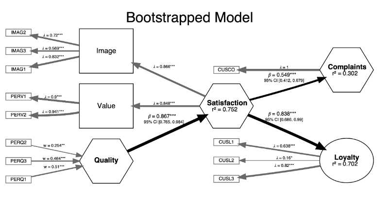
1 2	plot(boot_estimates, title = "Bootstrapped Model") save_plot("myfigure.png")

参考文献

https://cran.r-project.org/web/packages/seminr/vignettes/SEMinR.html
Yuan, K. H., & Bentler, P. M. (2000). Three likelihood-based methods for mean and covariance structure analysis with nonnormal missing data. Sociological methodology, 30(1), 165-200.
Zhao, X., Lynch Jr, J. G., & Chen, Q. (2010). Reconsidering Baron and Kenny: Myths and truths about mediation analysis. Journal of consumer research, 37(2), 197-206.

注意
统计咨询请加QQ 2726725926, 微信 shujufenxidaizuo, SPSS统计咨询是收费的, 不论什么模型都可以, 只限制于1个研究内.
跟我学统计可以代做分析, 每单几百元不等.
本文由jupyter notebook转换而来, 您可以在这里下载notebook
可以在微博上@mlln-cn向我免费题问
请记住我的网址: mlln.cn 或者 jupyter.cn

#amos #结构方程 #mplus #R

结构方程模型R语言实战教程

安装

数据

测量模型的设定

结构模型的设定

估计结果

Bootstrapping方法用于估计参数的显著性

汇报结果

描述性统计

参考文献

赞助

赞助推荐

常用工具

amos

结构方程

mplus

R

友商赞助